Greedy Programming
BACK: Dynamic Programming
Think of greedy programming as like a gradient descent method. We want to find a the correct direction of where we should go and then take a small step into that direction, in hopes that it will lead to a globally optimal solution. However, we may get stuck in a locally optimal solution.
Greedy algorithms often make assumptions and do not always yield optimal solutions, but for the problems we explore, they will.
Activity Selection Problem
Suppose you’re at some convention or something with several different events throughout the day, where some events will overlap with each other. We want to maximize the amount of activities we can fit in to our day, but without selecting incompatible activities.
We want to make the assumption that our activities are sorted in increasing order of their finish time:
\[\begin{array}{llllllllllll} i &| \quad 1 & 2 & 3 & 4 & 5 & 6 & 7 & 8 & 9 & 10 & 11 \\ s_i &| \quad 1 & 3 & 0 & 5 & 3 & 5 & 6 & 8 & 8 & 2 & 12 \\ f_i &| \quad 4 & 5 & 6 & 7 & 9 & 9 & 10 & 11 & 12 & 14 & 16 \end{array}\]A solution to this example (pg 415) is: \(\{a_1, a_4, a_8, a_{11}\}\). We can start with this problem by thinking about a dynamic programming solution–after all, the structure seems like it would have sub-solutions that can be stored into some table. (If we considered \(a_1\), what other best subsets could we make?).
The solution to the dynamic programming approach is on pg 416. But if we think even further than this: We could just pick the activities that leave the most amount of time for the rest of the activities, i.e: pick valid activities based on their increasing finishing times.
For this example, we can see that if we select \(a_1\), we can’t pick anything else until \(a_4\), since \(a_1\) finishes at 5. After picking \(a_4\), we can’t pick anything else until \(a_8\). And we can see that this is the solution to our problem: \(\{a_1, a_4, a_8, a_{11}\}\).
Making the greedy solution takes dynamic programming another step further. How can we start recursively, then just store our sub-solutions, and then make assumptions about our problem, so that it isn’t recursive at all? The linear pseudocode to this problem is on pg 421, but again assumes that we have sorted our finishing times in order.
Knapsack Problem
So what actually is the difference between dynamic programming and greedy algorithms? It’s a bit subtle and if you have a better way to explain it please let me know. The knapsack problem tries to demonstrate this.
If you were robbing a store and your knapsack could only carry \(w\) amount of weight–what should you steal in the store? Each item has a different price and weight.
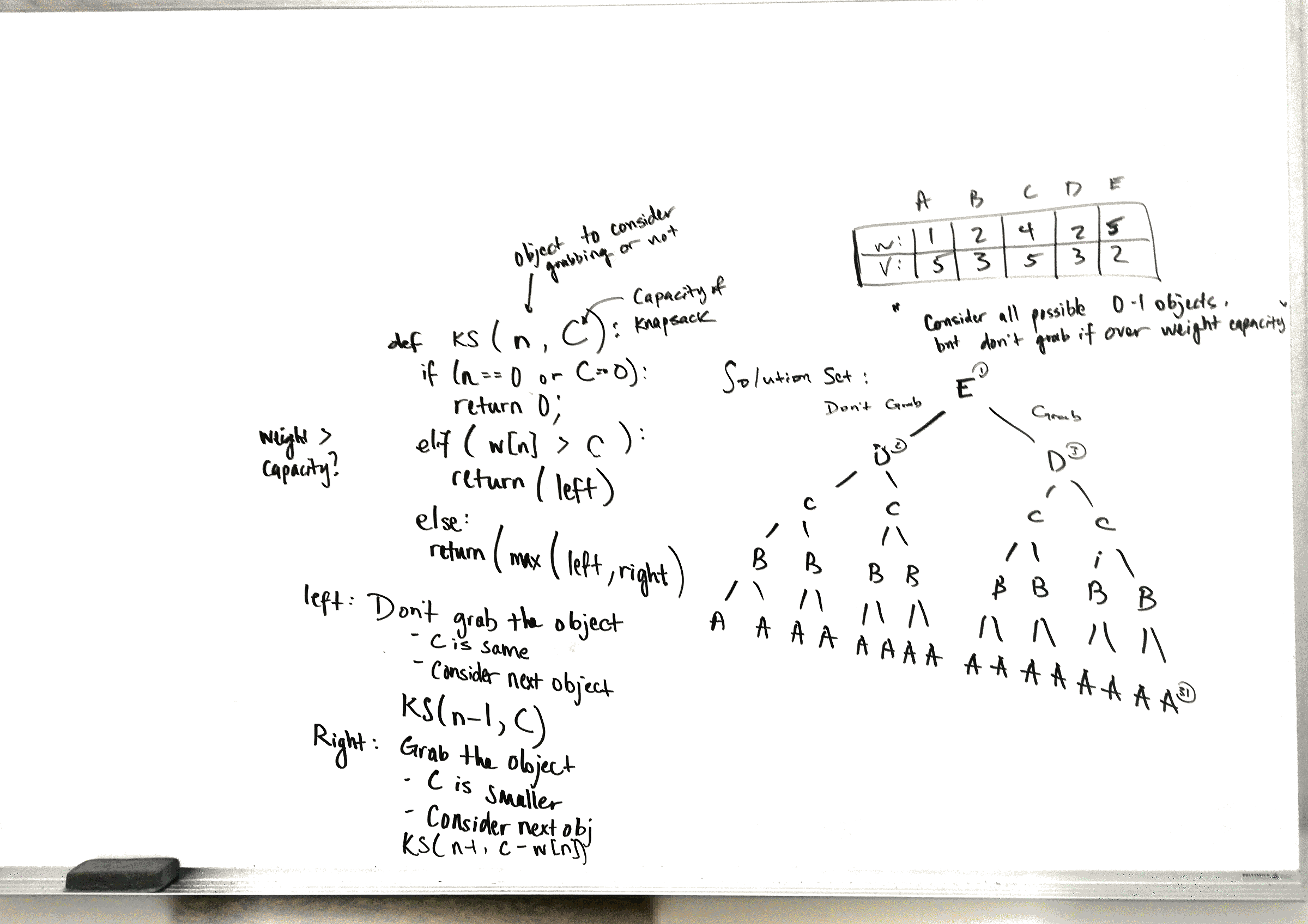
In the 0-1 Knapsack Problem, we can either take the item or leave it. Recursively, we might want to consider the first item–whether to take it or not, and then to recursively call the next item; making our tree look something like:

The solution space is \(O(2^n)\), as we have to consider every possibility and then select the max from each. But we can do better with dynamic programming.
For the 0-1 KS Problem, we aren’t able to apply a greedy solution. But suppose we could hold fractions of an item. i.e: Hold 66% of item 3. This is the fractional knapsack problem.
In this case, we can make several assumptions: Why would we not just fill up our knapsack all the way? On top of that? Why not just compute the value/weight ratio for every item and then pick based on their highest value/weights?
And that is the greedy solution to the fractional KS problem.
Huffman Coding
The aim of Huffman Coding is to compress the size of some text. If we have text with the characters \(\{a, b, c, d, e, f\}\), we could represent them with binary digits. Since we have 6 characters, we would need at least 3 bits to give each one a unique identifier, i.e:
Huffman coding is greedy in that we know how many times the characters are represented. It seeks to rearrange that tree in a different way such that the most used characters are placed closer up the tree than others–that way we can use less bits overall to represent the entire file.
If we organize the characters by their increasing frequencies, we can start building a Huffman tree from the bottom–the least used parts of the trees should be at the bottom. Each of these nodes can be “tree”ted as a Huffman Tree.
We can put all the frequencies into a minimum priority queue (whenever you pop the queue, you pop the element with the lowest value) and then start by popping the first two into a Huffman Tree. Afterwards, we can place that root of that tree back into the priority queue with a frequency of their combined frequencies. i.e:
Now the next two Huffman Trees in the queue are independent of the \(ef\) tree that we just made. This is fine–they will eventually converge to become part of the same tree. So now we will have two different parts of the tree, as so:
Now the next two trees in our queue are \(ef\) and \(d\). We can combine them to become a \(def\) tree like so:
Get it yet? We can continue this process until we use up all the nodes into one giant tree.
Eventually, we can conclude that the most optimal expression (least amount of bits for the given characters and frequencies) is the following: