Divide and Conquer
BACK: Data Structures
With most of the groundwork laid out, we can start discussing different algorithmic techniques: one of which are divide and conquer strategies.
We’ve already seen an example of the divide and conquer being used in merge sort. The big idea behind this strategy is to recursively divide up the problem into smaller subproblems and then conquer (solve) those subproblems before combining (merging) the solution back up together.
Maximum Sub-array Problem
The max subarray takes in an array and then computes the sum of the highest possible consecutive numbers. Examples:
Example 1:
- Input: [3, -2, 5, -1]
- Output: 6 ([3, -2, 5])
Example 2:
- Input: [3, -5, 2, 1, 4, -8, 6, 3]
- Output: 9 ([6, 3])
The idea is that we can split the array up in half until it has a size of 1: Any array with size 1 has a max sub-array of itself. To solve for the MSS, we have to consider 3 possibilities:
- The MSS is in the left side
- The MSS is in the right side
- The MSS crosses between the left and right side.
The first two cases are straightforward, but in the third case, we need to consider the max sum we can accumulate starting from the rightmost index of the left side and the max sum we can accumulate from the leftmost index of the right side–so that they connect. IE: Iterate through \(i = m\rightarrow 1\) and \(i = m + 1 \rightarrow q\) to find \(max(sum, sum + A[i])\)
To find the MSS of any recursive level, we want to take the max between the three possibilities. For the drawn out example of #2:
Analyzing Divide and Conquer
It’s a little harder to see the running time of a recursive function, but it is still doable. We know that every recursive function has to have an exit condition/base case. For something like fibnoacci, this is when we have input \(n = 0\) or \(n = 1\). For \(\text{Merge-Sort}\), this is when we have an input \(A\) with a size of 1.
Recurrences
For \(\text{Merge-Sort}\), we can see that we can just return the array itself once we get to the point where its size \(n = 1\). This is a constant time operation, so we say that when \(n = 1\), the time \(T(n)\) it takes to run the algorithm takes \(\theta(1)\) time.
Let’s now consider the next ideas. When we split up the array into two subproblems, they are of size \(\frac{n}{2}\). But we also have to consider the time it takes to divide the problem and the time it takes to combine the solved subproblems: \(D(n)\) and \(C(n)\) appropriately.
For \(\text{Merge-Sort}\), it takes a constant number of operations to divide the problem, so we have \(D(n) = \theta(1)\). To combine the subproblems, we have to iterate through the entirety of the subproblem, so that is \(\theta(n)\).
Through this analysis, we can see that the recurrence time for \(\text{Merge-Sort}\) takes:
\[T(n) = \left\{ \begin{array}{ll} \theta(1) & \quad \text{if } n = 1 \\ 2T(n/2) + \theta(n) & \quad \text{if } n > 1 \end{array} \right.\]Substitution Method
To use the substitution method in analyzing the runtime of an algorithm, we can provide a guess and then use induction to prove the our guess is correct.
ex: TBD
Recursion Tree Method
The recursion tree method helps us visualize the costs at each recursive level before we sum it all up together.
We need to consider several things here: the cost at each recursive level, the size of each subproblem, the number of subproblems (nodes).
Consider this example (pg 89):
\[T(n) = \left\{ \begin{array}{ll} \theta(1) & \quad \text{if } n = 1 \\ 3T(n/4) + cn^2 & \quad \text{if } n > 1 \end{array} \right.\]We start with the T(n). Other than our base case, we have \(T(n) = 3T(n/4) + cn^2\), meaning that we will have 3 subproblems of size \(\frac{n}{4}\). Also, to merge them together, we have a cost of \(cn^2\). We can draw it as the following:
We could add up the total runtime here, but it isn’t necessarily useful because we still haven’t hit the base case. We can continue expanding the problem this way, in order to find patterns to determine what the depth would be when eventually we converge to \(T(1)\). We can add up all the runtimes of \(T(n/4^i)\) (\(i\) for depth) and also include the runtime of our \(T(1)\)s. To get the total cost at each recursive level, we should multiply by how much one node costs by how many nodes there are in that recursive level.
Then we need to sum it all up together and find what the upper asymptotic bound should be.
Master Method
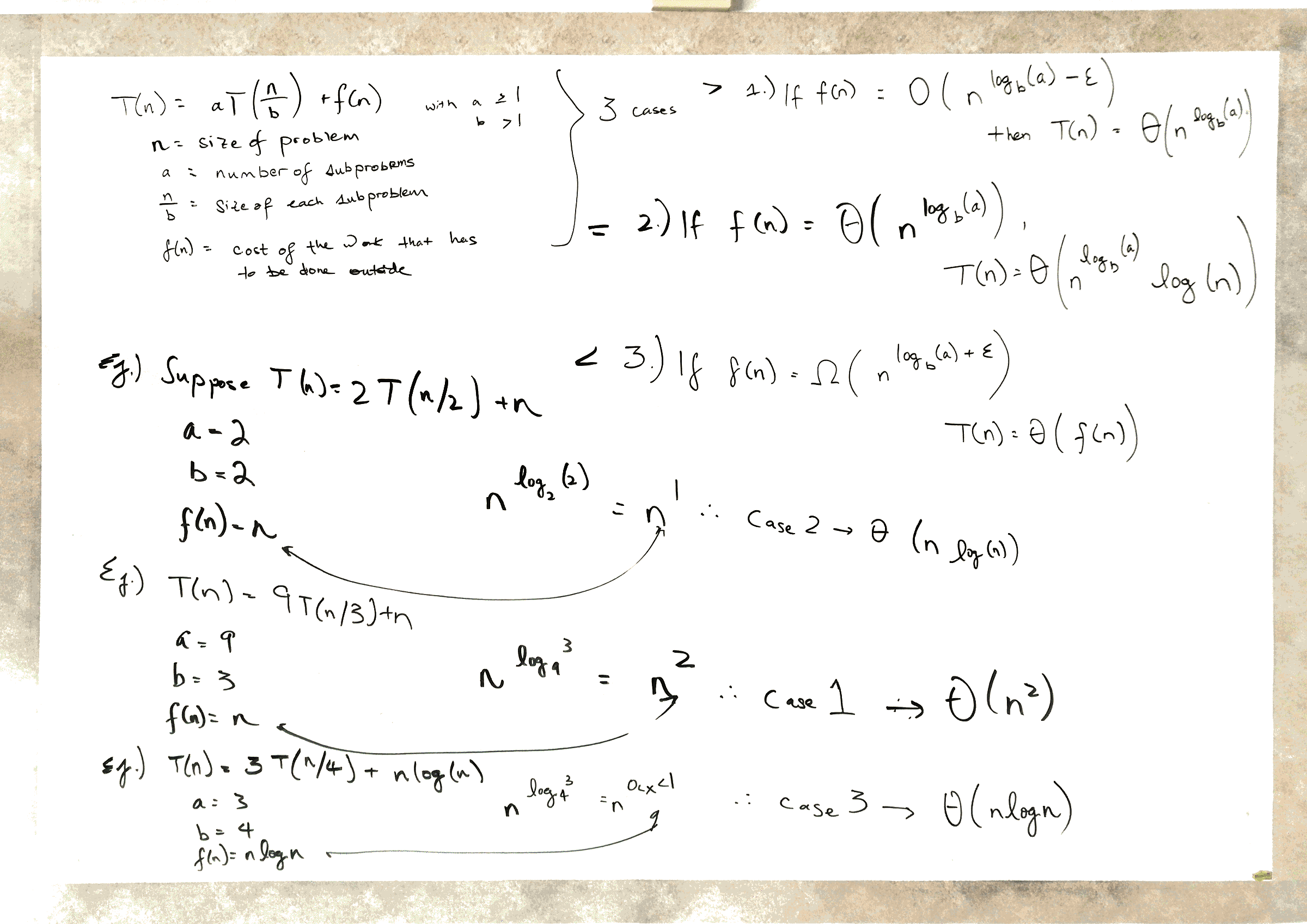
The master method can tell us what the runtime is for recurrences that take the following form:
\[T(n) = aT(\frac{n}{b}) + f(n) \text{, given that } a \geq 1, b > 1, \text{ and } f(n) \text{ is a function.}\]The following video explains it pretty well:
And these are the examples that he works out:
